こんにちは。sinyです。
この記事ではディープラーニングのライブラリの1つであるKerasの基本的な使い方について記載しています。
今のところはディープラーニング設計でKerasを利用しているのですが、たびたび利用方法を忘れていしまうことが多々あるため、備忘録としてKerasでよく扱う機能について使い方をまとめます。
(2020/4/5更新)
Kerasの基本構成
ワークフレームの方式
ディープラーニング開発のフレームワークにはいろいろな種類がありますが、Kerasは「Define-and-run」と呼ばれる方式のフレームワークです。
これは、ニューラルネットワークモデル構成を定義してからデータを投入するという方式です。
これは、データを投げながらニューラルネットワークモデルを定義するという方式でChainerとPytorchなどがこの方式を採用しています。
モデルの定義方法
Kerasにはニューラルネットワークモデルを定義する2つの方法があります。
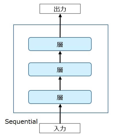
1つは「Sequentialクラス」を利用する方法、もう1つは「Functional API」を利用する方法です。
Sequentialクラスは入力と出力が必ず1つずつのネットワーク構成しか定義することができません。
また、中間の層内でネットワークを分岐させるような構成も作れません。(層の線形スタック構成)
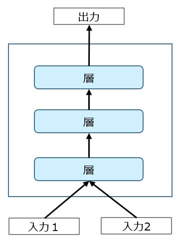
一方、Functional APIは完全カスタムなネットワーク構成を定義することができます。
入力が2つ、出力が1つといったネットワークを定義することができます。
Kerasの基本機能
Sequentialモデル
モデル定義
Sequentialモデル定義の基本的な例
#学習鵜モデルの定義
from keras import layers
from keras import models


model = models.Sequential()
model.add(Dense(10, activation='relu', input_shape=(4,)))
model.add(Dense(3, activation='softmax'))
上記は以下のニューラルネットワークモデルを定義したことになります。

| 要素 | 説明 |
| Dense(keras.layers.Dense) | Denseとは全結合ニューラルネットワークで、1つのニューラルネットワークを定義する。 |
| model = keras.models.Sequential() | シーケンシャル(順番に)モデルを追加するモデルを定義する。 |
| model.add(Dense(10, activation='relu', input_shape=(4,))) | mode.addでモデルに定義を順番に追加していく。 input_shape=入力するデータの次元数は最初の層だけに指定する。 |
| model.add(Dense(3, activation='softmax')) | Dense()の引数には、Dense(ユニット数, activation='活性化関数')を指定する。 |
- モデルの最初のレイヤには入力のshapeについて情報を指定する必要がある。
※input_shape引数:shapeを示すタプルを指定(整数 ro None)
※Noneを指定すると任意の整数
※Dense のような2次元の層では input_dim引数を指定することで入力のshapeを指定できる。
※3次元のレイヤーでは input_dim引数と input_length引数を指定することで入力のshapeを指定
※batch_size=32と input_shape=(6, 8)を同時に指定した場合,想定されるバッチごとの入力のshapeは (32, 6, 8)となる。 - Input_shapeの指定の仕方
① model.add(Dense(32, input_shape=(784,)))
② model.add(Dense(32, input_dim=784))
上記①,②は同じこと。
モデル構造のコンパイル
基本的にモデルのcompileには3つの引数を指定する。
サンプルコード
from keras import optimizers

model.compile(loss='categorical_crossentropy',
              optimizer='rmsprop',
              metrics=['acc'])
- lossで損失関数を指定
- optimizerに最適化アルゴリズムを指定
- 評価関数のリスト
損失関数
損失関数の選択の目安(一般的に役立つ可能性がある組み合わせ)
| 問題の種類 | 損失関数 |
| 二値分類 | binary_crossentropy |
| 多クラス単一ラベル分類 | categorical_crossentropy |
| 多クラス多ラベル分類 | binary_crossentropy |
| 回帰問題(任意の値) | mse |
| 回帰問題(0~1の値) | mse / binary_crossentropy |
学習の実行
学習はfitメソッドで実行する。
model.fit(x_train, y_train,
    batch_size=20,
    epochs=300)
- model.fit(入力データ,正解ラベル, バッチサイズ、エポック数)
- バッチサイズを小さくすると消費メモリが少なくて済むが、うまく動かなくなる。
- エポックは学習の繰り返す数
- fitメソッドの戻り値 History オブジェクト. History.history 属性は 実行に成功したエポックにおける訓練の損失値と評価関数値の記録と,(適用可能ならば)検証における損失値と評価関数値も記録される。
- loss
→学習データでの損失値 - va_loss
→検証データでの損失値 - acc
→学習データでの正解率 - val_acc
→検証データでの正解率 - lossとval_lossは以下のように抽出できる。
<model>.history['loss'] <model>.history['val_loss']
モデルの評価
モデルの評価はevaluateメソッドを使う。
サンプルコード
score = model.evaluate(x_test, y_test, verbose=1
print('正解率=', score[1], 'loss=', score[0]
- evaluate(入力データ, 出力データ, batch_size,verbose=1or0,sample_weight, steps)
※バッチサイズはデフォルト32
※verboseは進行状況メッセージ出力モードで,0か1.
※sample_weight: サンプルの重み
※steps: 整数またはNone.評価ラウンド終了を宣言するまでの総ステップ数(サンプルのバッチ) - model.evaluateメソッドの戻り値
test_loss, test_acc = model.evaluate(test_images, test_labels)
※test_loss:損失%
※test_acc:精度%
モデルの保存とロード
学習したモデルはファイルへ保存、ファイルからロードができる。
from keras.models import load_model
model.save('****.h5')
model = load_model('****.h5')
重みの保存とロード
重みの保存とロードは以下のように実施できます。
model.save_weights('param.hdf5')  #保存

model.load_weights('param.hdf5')  #ロード
重みの確認
重みをロードした場合に以下のようなエラーが発生する場合があります。
この場合は、定義されたモデルのレイヤーと保存された重みのレイヤーが異なっている可能性があるので、各レイヤーがどうなっているか確認してみるとよいです。
定義済みモデルの重みは<モデル名>.weightsで確認できます。
discriminator.weights

[<tf.Variable 'conv2d_13/kernel:0' shape=(3, 3, 3, 32) dtype=float32_ref>, <tf.Variable 'conv2d_13/bias:0' shape=(32,) dtype=float32_ref>, <tf.Variable 'conv2d_14/kernel:0' shape=(3, 3, 32, 64) dtype=float32_ref>, <tf.Variable 'conv2d_14/bias:0' shape=(64,) dtype=float32_ref>, <tf.Variable 'batch_normalization_18/gamma:0' shape=(64,) dtype=float32_ref>, <tf.Variable 'batch_normalization_18/beta:0' shape=(64,) dtype=float32_ref>, <tf.Variable 'conv2d_15/kernel:0' shape=(3, 3, 64, 128) dtype=float32_ref>, <tf.Variable 'conv2d_15/bias:0' shape=(128,) dtype=float32_ref>, <tf.Variable 'batch_normalization_19/gamma:0' shape=(128,) dtype=float32_ref>, <tf.Variable 'batch_normalization_19/beta:0' shape=(128,) dtype=float32_ref>, <tf.Variable 'dense_8/kernel:0' shape=(8192, 1) dtype=float32_ref>, <tf.Variable 'dense_8/bias:0' shape=(1,) dtype=float32_ref>, <tf.Variable 'batch_normalization_18/moving_mean:0' shape=(64,) dtype=float32_ref>, <tf.Variable 'batch_normalization_18/moving_variance:0' shape=(64,) dtype=float32_ref>, <tf.Variable 'batch_normalization_19/moving_mean:0' shape=(128,) dtype=float32_ref>, <tf.Variable 'batch_normalization_19/moving_variance:0' shape=(128,) dtype=float32_ref>]
save_weightsメソッドで保存したhdf5の中身を確認するには以下のコードを実行します。
import h5py
model_weights = h5py.File(<重みのファイル名>.hdf5', 'r')
print(model_weights.keys())

<KeysViewHDF5 ['activation_3', 'batch_normalization_15', 'batch_normalization_16', 'batch_normalization_17', 'conv2d_transpose_10', 'conv2d_transpose_11', 'conv2d_transpose_12', 'conv2d_transpose_9', 'dense_7', 'leaky_re_lu_19', 'leaky_re_lu_20', 'leaky_re_lu_21', 'reshape_3']>
画像データ(CNN)の扱い
画像データを扱う場合は通常2次元のConv2D層を利用します。
- model.add(Conv2D(フィルタ数,フィルタサイズ,入力データ)
※filters=32,kernel_size=3, input_shape=(256,256,3)という感じに書く。
※model.add(Conv2D(Output_depth,(window_height,window_width))
※例)model.add(Conv2D(32,(3,3), activation="relu",input_shape=(28,28,1))))
28x28のグレースケール画像を3*3フィルタで畳み込んで
(height,width,outputh=32)の3次元の出力特徴マップを生成
※padding: "valid"か"same"のどちらかを指定。(デフォルトはvalid=paddingなし)
※Conv2Dの入力は、(image_height, image_width, image_channels)という形状にする必要がある。
→(バッチの次元を含まない)
※モノクロなら (28, 28, 1)、カラーならカラーなら(28,28, 3)のように指定する。 - model.add(MaxPooling2D(pool_size=2,2)))
※Maxプーリング(2x2)の場合の定義
※パラメータは2つ、 pool_size, strides(省略するとpool_sizeと同じに設定)
※他にはAveragePoolingという手法もある。(https://keras.io/layers/pooling/) - model.add(Flatten())
※多次元配列を1次元のベクトルに変換してくれるもの
分散表現
Embeddingはオブジェクトをベクトルにマップするので、アプリケーションはベクトル空間における類似性 (e.g., ユークリッド距離やベクトル間の角度) をオブジェクトの類似性の堅牢で柔軟な尺度として利用できる。
- Embedding(正の整数(インデックス)を固定次元の密ベクトルに変換する)
例)model.add(Embedding(20,10, input_length=5)) - 自然言語での使い方
Embedding(語彙数, 分散ベクトルの次元数, 文書の次元数))
※事前に入力文書の次元数をそろえる必要がある。
※model.add(Embedding(20,10, input_length=5))
→入力長5、語録数20、分散ベクトルを10次元として、入力から出力(分散ベクトル10)を出力する。 - Embeddingレイヤーはモデルの最初のレイヤーとしてのみ利用できる。
Tokenizer
テキストをベクトル化する、またはテキストをシーケンス化してくれるクラス。
サンプルコード
text = "I love green eggs and ham ."
tokenizer = Tokenizer()
tokenizer.fit_on_texts()
#fit_on_textsメソッドを通した後に、word_indexメソッドで抽出すると、以下の通り単語とそのIDの変換を行ってくれる。
tokenizer.word_index
Out[12]:
{'and': 5, 'eggs': 4, 'green': 3, 'ham': 6, 'i': 1, 'love': 2}
※辞書型のデータ(単語トークンのリスト)が生成される。{単語:キー}
One-hot表現への変換
ある値をOne-hot表現に変換したい場合にKerasのto_categoricalが便利です。
第1引数にリスト形式のデータ、num_classesにOne-hot表現の数を指定します。
以下、参考例です。
from keras.utils import to_categorical
test = [0,5,3,2,2,9,3,3,2,1]
one_hot = to_categorical(test, num_classes=10)
print(one_hot)


[[1. 0. 0. 0. 0. 0. 0. 0. 0. 0.]
 [0. 0. 0. 0. 0. 1. 0. 0. 0. 0.]
 [0. 0. 0. 1. 0. 0. 0. 0. 0. 0.]
 [0. 0. 1. 0. 0. 0. 0. 0. 0. 0.]
 [0. 0. 1. 0. 0. 0. 0. 0. 0. 0.]
 [0. 0. 0. 0. 0. 0. 0. 0. 0. 1.]
 [0. 0. 0. 1. 0. 0. 0. 0. 0. 0.]
 [0. 0. 0. 1. 0. 0. 0. 0. 0. 0.]
 [0. 0. 1. 0. 0. 0. 0. 0. 0. 0.]
 [0. 1. 0. 0. 0. 0. 0. 0. 0. 0.]]
重みの正規化
KerasでL2正規化を適用する例
# 重みにL2正規化を適用したモデル
from keras import regularizers

l2_model = models.Sequential()
l2_model.add(layers.Dense(16, kernel_regularizer=regularizers.l2(0.001),
                          activation='relu', input_shape=(10000,)))
l2_model.add(layers.Dense(16, kernel_regularizer=regularizers.l2(0.001),
                          activation='relu'))
l2_model.add(layers.Dense(1, activation='sigmoid'))
- kernel_regularizer=regularizers.l2(0.001)
→該当層の重み行列の係数ごとにネットワークの全損失に0.001*weight_coefficient_valueを足すことを意味している。 - weight_coefficient_value=重み系数値
- 同様にL1正規化を適用、L1,L2を同時に適用することもできる。
- L1正規化を適用する場合
→ kernel_regularizer=regularizers.l1(0.001) - L1,L2正規化を同時適用する場合
→regularizer=regularizers.l1_l2(l1=0.001,l2=0.001),
Dropアウト
通常Dropアウト率は0.2~0.5に設定する。
KerasでのDropアウトの適用例
model.add(layers.Dropout(0.5))
Keras functional API
Functional APIは定義した層を任意に連結できる。
層の定義の最後に連結したい層の名前を()付きで書くと層が連結されていく。
input_1 = Input(shape=(None,))
name_2 = layers.Embedding()(input_1)
name_3 = layers.LSTM(32)(name_2)
name_4 = layers.LSTM(32)(name_3)
2つの入力を元にLSTM層に入力して、結合して1つの出力を得るモデル定義の例
from keras import Model
from keras import layers
from keras import Input
#入力Aを定義
input_a = Input(shape=(None,), name="input_a")
#入力Aを畳み込み
embedded_a = layers.Embedding(1000,64)(input_a)
#入力AをLSTMでエンコード
encoded_a = layers.LSTM(32)(embedded_a)

#入力Bを定義
input_b = Input(shape=(None,), name="input_b")
#入力Bを畳み込み
embedded_b = layers.Embedding(1000,64)(input_b)
#入力BをLSTMでエンコード
encoded_b = layers.LSTM(32)(embedded_b)

#emcoded_aとencoded_bを結合
concatenated = layers.concatenate([encoded_a , encoded_b], axis=-1)
#出力層を定義
output = layers.Dense(500, activation="softmax")(concatenated)

#モデル全体の定義(リスト形式で複数の入力を指定する)
model = Model([input_a, input_b], output)
model.compile(optimizer="rmsprop",
             loss="categorical_crossentropy",
             metrics=["acc"])
上記コードは、以下のネットワークを定義したことになる。

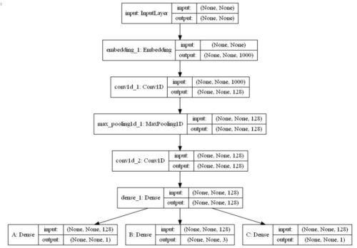
単一入力、多出力モデルの例
入力が1つ、A,B,C3つの出力を行うモデル定義の例
input = Input(shape=(None,),name="input")
embedded_input = layers.Embedding(256, 1000)(input)
x = layers.Conv1D(128,5 ,activation="relu")(embedded_input)
x = layers.MaxPooling1D(5)(x)
x = layers.Conv1D(128,5 ,activation="relu")(x)
x = layers.Dense(128, activation="relu")(x)

A = layers.Dense(1, name="A")(x)
B = layers.Dense(3,activation="softmax",name="B")(x)
C = layers.Dense(1, activation="sigmoid",name="C")(x)
model = Model(input,[A,B,C])

model.compile(optimizer="rmsprop",
             loss=["mse", "categorical_crossentropy", "binary_crossentropy"])
モデルのネットワークは以下の通り。
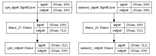
オートエンコーダで2入力、2出力を定義した場合の例
入力も出力も複数ある場合は、
autoencoder = Model([cpu_input, memory_input], [decoded_cpu, decoded_memory])
のようにリストで入力、出力層の定義名を指定すればよい。
w_size = 100 # ウィンドウサイズ
l1=10e-7  # L1正則化のパラメータ
enc_dim = 512  # 隠れ層のユニット数

cpu_input = Input(shape=(w_size,),name="cpu_input")
encoded_cpu = Dense(enc_dim, activation='relu',
                activity_regularizer=regularizers.l1(l1))(cpu_input)
decoded_cpu = Dense(w_size, activation='relu',name="cpu_output")(encoded_cpu)

memory_input = Input(shape=(w_size,),name="memory_input")
encoded_memory = Dense(enc_dim, activation='relu',
                activity_regularizer=regularizers.l1(l1))(memory_input)
decoded_memory = Dense(w_size, activation='relu',name="memory_output")(encoded_memory)


autoencoder = Model([cpu_input, memory_input], [decoded_cpu, decoded_memory])
autoencoder.compile(optimizer='adadelta',
                    loss=['binary_crossentropy', 'binary_crossentropy'])
ネットワーク図は以下の通り。
トレーニングは、fitメソッドの入力、ラベル部分にリスト形式でデータを指定すればよい。
# モデルの学習
early_stopping = EarlyStopping(patience=2, verbose=1)


epochs = 1000
history = autoencoder.fit([X_train_cpu,X_train_mem],
                          [X_train_cpu,X_train_mem],
                          epochs=epochs,
                          batch_size=None,
                          verbose=1,
                          callbacks=[early_stopping])
その他
pad_sequences
シーケンスを同じ長さになるように詰めてくれる機能。
- padding: 文字列,'pre'または'post'.各シーケンスの前後どちらを埋めるか.
- truncating: 文字列,'pre'または'post'.
maxlenより長いシーケンスの前後どちらを切り詰めるか.
※参考コード
a1 = [1,2,3,4]
a2 = [1,2,3,4,5,6,7,8,9,10]
print(pad_sequences([a1], maxlen=8, padding='pre', truncating='pre')[0])
print(pad_sequences([a1], maxlen=8, padding='post', truncating='pre')[0])
print(pad_sequences([a1], maxlen=8, padding='pre', truncating='post')[0])
print(pad_sequences([a1], maxlen=8, padding='post', truncating='post')[0])
print(pad_sequences([a2], maxlen=8, padding='pre', truncating='pre')[0])
print(pad_sequences([a2], maxlen=8, padding='post', truncating='pre')[0])
print(pad_sequences([a2], maxlen=8, padding='pre', truncating='post')[0])
print(pad_sequences([a2], maxlen=8, padding='post', truncating='post')[0])

#実行結果

[0 0 0 0 1 2 3 4]
[1 2 3 4 0 0 0 0]
[0 0 0 0 1 2 3 4]
[1 2 3 4 0 0 0 0]
[ 3  4  5  6  7  8  9 10]
[ 3  4  5  6  7  8  9 10]
[1 2 3 4 5 6 7 8]
[1 2 3 4 5 6 7 8]
こちらの記事も参考になります。
パラメータの固定化
訓練時にパラメータを工程にして更新されないようにするにはモデルのtrainable属性をFalseに設定する。
<モデル名>.trainable = False
なお、モデルをcompile後にtrainbale属性を変更した場合は、設定を反映させるために再度compileする必要がある。