
こんにちは。sinyです。
最近GANについて学習していますが、深層畳み込みGAN(DCGAN)を実装した際の情報を記事にまとめました。
前提として以下のGANの関連記事を読んでおくと理解しやすいと思います。

本記事では下記Githubリポジトリをベースにコードを作っています。
また、書籍などでは大体MNISTデータをコマンド一発でロードして学習させるパターンが多いですが、実際に利用する場合は個別の画像ファイルを読み込む形で実装する必要があるので、Googleドライブ上に準備したねこ画像500枚をランダムにロードして学習させる形のサンプルコードを作りました。
さらにGANでは学習に時間がかかるのでGoogle Corabo上でも実行制限にかかって最後まで学習ができませんので、500エポック毎にパラメータをGoogleドライブ上に保存する形にしています。
DCGANとは?
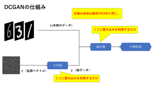
最もシンプルなGANでは生成器と識別器に単純な2層のFeedForwardネットワーク(全結合層とかDenseなどといったりもする)を使いますが、ここに畳み込みニューラルネットワーク(CNN)を用いたものがDCGANです。(下図参照)
DCGANの識別器
下図の通り、識別器のネットワークにCNNを用います。
以下の例では28 x 28 x 1のモノクロ画像を入力として畳み込みを数回実行します。
基本的にバッチ正則化→活性化関数(LeackyReLU)を適用しています。(最初の畳み込みの後は活性化のみ)
最後に入力された画像が本物(1)or 偽物(0)を識別できるようにシグモイド関数をかまして0~1に変換してあげます。
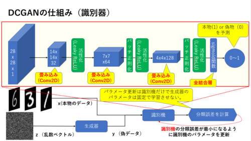
図にも書いてありますが、識別機の学習の際は生成器側のパラメータを更新しないように固定させ、識別器側のネットワークパラメータだけ学習させます。
この点は通常のGANと同じです。
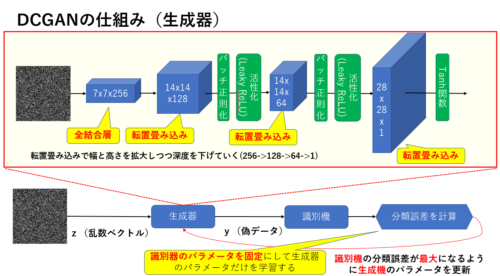
DCGANの生成器
生成器も識別器と同様にCNNを適用していきますが、こちらは乱数ベクトルから画像を生成するため通常のCNNではなく転置畳み込みを利用しています。
例えばkerasだとConv2DTransposeを使って簡単に実装できます。
生成器では転置畳み込みで幅と高さを拡大しつつ深度を徐々に下げていきます(256->128-> 64->1)。
サンプルコード
全コードは下記リポジトリからダウンロードできます。
以下、要点だけ解説していきます。
Tensorflowのバージョンを変更する
2020年4月14日現在、Google CoraboのデフォルトのTensorflowバージョンがtensorflow-2.2.0rc2になっていますが、このバージョンだとうまく動作しないので、1.14.0にダウングレードします。
pip install TensorFlow==1.14
その後、以下のコードでGoogleドライブをマウントします。
from google.colab import drive
drive.mount('/content/drive')
必要なライブラリーをインポートします。
%matplotlib inline

import matplotlib.pyplot as plt
import numpy as np
import os
from keras.datasets import mnist
from keras.layers import Activation, BatchNormalization, Dense, Dropout, Flatten, Reshape
from keras.layers.advanced_activations import LeakyReLU
from keras.layers.convolutional import Conv2D, Conv2DTranspose
from keras.models import Sequential
from keras.optimizers import Adam
from keras.preprocessing.image import load_img, img_to_array, array_to_img
#モデルの可視化
#from tensorflow.python.keras.utils.vis_utils import plot_model

from keras.utils.vis_utils import plot_model
from keras.models import load_model
import glob
今回は、64 x 64のカラー画像を扱うので以下のように設定します。
また、生成器では100次元のベクトルから画像を生成することとします。
img_rows = 64
img_cols = 64
channels = 3

# 入力画像の形状(64 x 64 x 3) //カラー画像
img_shape = (img_rows, img_cols, channels)

# noiseベクトルサイズ(生成器へのINPUT)
z_dim = 100
生成器の定義は以下の通りです。
ef build_generator(z_dim):

    model = Sequential()

    #  全結合層によってnoiseベクトル(200次元)をReshapeして7x7x256 tensorに変換する
    model.add(Dense(256 * 8 * 8, input_dim=z_dim))
    model.add(Reshape((8, 8, 256)))

    # 転置畳み込みにより8x8x256 から 16x16x128テンソルに変換
    model.add(Conv2DTranspose(128, kernel_size=3, strides=2, padding='same'))

    # バッチ正規化
    model.add(BatchNormalization())

    # Leaky ReLU活性化
    model.add(LeakyReLU(alpha=0.01))

    # 転置畳み込みにより16x16x128 から 32x32x64テンソルに変換
    model.add(Conv2DTranspose(128, kernel_size=3, strides=2, padding='same'))

    # バッチ正規化
    model.add(BatchNormalization())

    # Leaky ReLU活性化
    model.add(LeakyReLU(alpha=0.01))

    # 転置畳み込みにより32x32x64 から32x32x32 テンソルに変換
    model.add(Conv2DTranspose(64, kernel_size=3, strides=1, padding='same'))

    # バッチ正規化
    model.add(BatchNormalization())

    # Leaky ReLU活性化
    model.add(LeakyReLU(alpha=0.01))

    # Transposed convolution layer, from 32x32x32 to 64x64x3 tensor
    model.add(Conv2DTranspose(3, kernel_size=3, strides=2, padding='same'))

    # tanh活性化を適用して出力(最終層だけはバッチ正規化はしない)
    model.add(Activation('tanh'))

    return model
以下のコードを実行してモデルを可視化しています。
build_model = build_generator(z_dim)

plot_model(build_model, to_file="DCGAB_build_model.png", show_shapes=True)
続いて識別機の定義です。
def build_discriminator(img_shape):

    model = Sequential()

    # 64x64x3(入力画像) を32x32x32のテンソルにする畳み込み層
    model.add(
        Conv2D(32,
               kernel_size=3,
               strides=2,
               input_shape=img_shape,
               padding='same')) #padding=sameにすると、入力の大きさをstridesの大きさで単純に割ったもの(28/2=14)が出力の大きさになる

    # Leaky ReLUによる活性化(最初の層にはバッチ正規化は適用しない)
    model.add(LeakyReLU(alpha=0.01))

    # 32x32x32 を16x16x64のテンソルにする畳み込み層
    model.add(
        Conv2D(64,
               kernel_size=3,
               strides=2,
               input_shape=img_shape,
               padding='same'))

    # バッチ正規化
    model.add(BatchNormalization())

    # Leaky ReLUによる活性化
    model.add(LeakyReLU(alpha=0.01))

    # 16x16x64 を8x8x128のテンソルにする畳み込み層
    model.add(
        Conv2D(128,
               kernel_size=3,
               strides=2,
               input_shape=img_shape,
               padding='same'))

    # バッチ正規化
    model.add(BatchNormalization())

    # Leaky ReLU活性化
    model.add(LeakyReLU(alpha=0.01))

    # シグモイド関数で出力(0~1)
    model.add(Flatten())
    model.add(Dense(1, activation='sigmoid'))

    return model


def build_gan(generator, discriminator):

    model = Sequential()

    # 生成器と識別機を結合
    model.add(generator)
    model.add(discriminator)

    return model
生成器と識別機のコンパイルをします。
# 識別機の生成とコンパイル
discriminator = build_discriminator(img_shape)
discriminator.compile(loss='binary_crossentropy',
                      optimizer=Adam(),
                      metrics=['accuracy'])

#前回学習の重みをロード
discriminator.load_weights('/content/drive/My Drive/Colab Notebooks/GAN/models/D/d_param-50490.hdf5')


# 生成器の生成
generator = build_generator(z_dim)

# 生成器の訓練時は識別機のパラメータを固定する
discriminator.trainable = False

# 識別機は固定のまま生成器を訓練するGANモデルの生成とコンパイル
gan = build_gan(generator, discriminator)
gan.compile(loss='binary_crossentropy', optimizer=Adam())
なお、以下の部分で直近の学習完了時に生成された識別機のパラメータファイル(d_param-50490.hdf5)をロードします。
※パスとファイル名のところは適宜変更してください。
discriminator.load_weights('/content/drive/My Drive/Colab Notebooks/GAN/models/D/d_param-50490.hdf5')
また生成器についても直近の学習完了時に生成されたパラメータファイルをロードします。
こちらもパスとファイル名は適宜変更してください。
#途中までの学習済みモデルのロード
from keras.models import load_model

model_g_dir = "/content/drive/My Drive/Colab Notebooks/GAN/models/G"
model_d_dir = "/content/drive/My Drive/Colab Notebooks/GAN/models/D"

#generator = load_model('/content/drive/My Drive/Colab Notebooks/GAN/models/G/g_model-2499.h5')
generator.load_weights('/content/drive/My Drive/Colab Notebooks/GAN/models/G/g_param-50490.hdf5')


#gan = load_model('/content/drive/My Drive/Colab Notebooks/GAN/models/D/d_model-2499.h5')
gan.load_weights('/content/drive/My Drive/Colab Notebooks/GAN/models/G/gan_param-50490.hdf5')
訓練メソッドの定義は以下の通りです。
losses = []
accuracies = []
iteration_checkpoints = []
train_dir = "/content/drive/My Drive/Colab Notebooks/GAN/data/cats"
output_dir = "/content/drive/My Drive/Colab Notebooks/GAN/data/result"
model_g_dir = "/content/drive/My Drive/Colab Notebooks/GAN/models/G"
model_d_dir = "/content/drive/My Drive/Colab Notebooks/GAN/models/D"
height = 64
width = 64
num_of_trials = 50490


def train(iterations, batch_size, sample_interval, files):
  arrlist = []
  for i, imgfile in enumerate(files):
    img = load_img(imgfile, target_size=(height, width))    # 画像ファイルの読み込み
    array = img_to_array(img)    # 画像ファイルのnumpy化
    arrlist.append(array)    # numpy型データをリストに追加
    print("ファイルINDEX=", i)
  # ndary型に変換
  X_train = np.array(arrlist)   # (2000, 64, 64, 3)

  # Rescale [0, 255] grayscale pixel values to [-1, 1]
  X_train = X_train / 127.5 - 1.0


  # Labels for real images: all ones
  real = np.ones((batch_size, 1))

  # Labels for fake images: all zeros
  fake = np.zeros((batch_size, 1))
  print("check-001")

  for iteration in range(iterations):

      # -------------------------
      #  Train the Discriminator
      # -------------------------
      print("iteration=", iteration)

      # Get a random batch of real images
      idx = np.random.randint(0, X_train.shape[0], batch_size)
      imgs = X_train[idx]
       # Generate a batch of fake images
      z = np.random.normal(0, 1, (batch_size, 100))
      gen_imgs = generator.predict(z)
       # Train Discriminator


      d_loss_real = discriminator.train_on_batch(imgs, real)
      d_loss_fake = discriminator.train_on_batch(gen_imgs, fake)
      d_loss, accuracy = 0.5 * np.add(d_loss_real, d_loss_fake)


      # ---------------------
      #  Train the Generator
      # ---------------------

      # Generate a batch of fake images
      z = np.random.normal(0, 1, (batch_size, 100))
      gen_imgs = generator.predict(z)

      # Train Generator
      g_loss = gan.train_on_batch(z, real)

      if (iteration + 1) % sample_interval == 0:

          # Save losses and accuracies so they can be plotted after training
          losses.append((d_loss, g_loss))
          accuracies.append(100.0 * accuracy)
          iteration_checkpoints.append(iteration + 1)

          # Output training progress
          print("%d [D loss: %f, acc.: %.2f%%] [G loss: %f]" %
                (iteration + 1, d_loss, 100.0 * accuracy, g_loss))

          # Output a sample of generated image
          sample_images(generator, iteration)
          #識別器のモデル保存
          d_model_file=os.path.join(model_d_dir, "d_model-" + str(iteration + num_of_trials) +  ".h5")
          d_param_file=os.path.join(model_d_dir, "d_param-" + str(iteration + num_of_trials) +  ".hdf5")
          discriminator.save(d_model_file)
          discriminator.save_weights(d_param_file)

          #生成器のモデル保存
          g_model_file=os.path.join(model_g_dir, "g_model-" + str(iteration + num_of_trials) +  ".h5")
          g_param_file=os.path.join(model_g_dir, "g_param-" + str(iteration + num_of_trials) +  ".hdf5")
          generator.save(g_model_file)
          generator.save_weights(g_param_file)
          gan_model_file=os.path.join(model_g_dir, "gan_model-" + str(iteration + num_of_trials) +  ".h5")
          gan_param_file=os.path.join(model_g_dir, "gan_param-" + str(iteration + num_of_trials) +  ".hdf5")

          gan.save(gan_model_file)
          gan.save_weights(gan_param_file)
以下の部分でsample_interval変数で指定したエポック毎にモデルパラメータをGoogleドライブ上に保存するようにしています。
          #識別器のモデル保存
          d_model_file=os.path.join(model_d_dir, "d_model-" + str(iteration + num_of_trials) +  ".h5")
          d_param_file=os.path.join(model_d_dir, "d_param-" + str(iteration + num_of_trials) +  ".hdf5")
          discriminator.save(d_model_file)
          discriminator.save_weights(d_param_file)

          #生成器のモデル保存
          g_model_file=os.path.join(model_g_dir, "g_model-" + str(iteration + num_of_trials) +  ".h5")
          g_param_file=os.path.join(model_g_dir, "g_param-" + str(iteration + num_of_trials) +  ".hdf5")
          generator.save(g_model_file)
          generator.save_weights(g_param_file)
          gan_model_file=os.path.join(model_g_dir, "gan_model-" + str(iteration + num_of_trials) +  ".h5")
          gan_param_file=os.path.join(model_g_dir, "gan_param-" + str(iteration + num_of_trials) +  ".hdf5")

          gan.save(gan_model_file)
          gan.save_weights(gan_param_file)
また、以下の部分で生成した画像を表示してGoogleドライブに保存するメソッドを呼び出しています。
# Output a sample of generated image
sample_images(generator, iteration)
sample_imagesメソッドは以下の通りです。
def sample_images(generator, iteration, image_grid_rows=4, image_grid_columns=4):

    # Sample random noise
    z = np.random.normal(0, 1, (image_grid_rows * image_grid_columns, z_dim))

    # Generate images from random noise
    gen_imgs = generator.predict(z)  # (16, 64, 64, 3)

    # Rescale image pixel values to [0, 1]
    gen_imgs = 0.5 * gen_imgs + 0.5

    # Set image grid
    fig, axs = plt.subplots(image_grid_rows,
                            image_grid_columns,
                            figsize=(4, 4),
                            sharey=True,
                            sharex=True)
    #print("gen_imgs_shape=", gen_imgs.shape)
    #print("gen_imgs_type=", type(gen_imgs.shape))
    #print("gen_imgs_shape2=", gen_imgs[0,:,:,:].shape)
    cnt = 0
    for i in range(image_grid_rows):
        for j in range(image_grid_columns):
            # Output a grid of images
            #print("shape=",gen_imgs[cnt, :, :, :].shape)
            axs[i, j].imshow(gen_imgs[cnt, :, :, :])
            axs[i, j].axis('off')
            cnt += 1
    #file保存
    output_file = os.path.join(output_dir, 'result_' + str(iteration + num_of_trials) +'.png')
    plt.savefig(output_file)
最後に学習を開始します。
以下の例では、学習を5000エポック行い500エポック毎に生成画像を表示して、モデルパラメータを保存するようにしています。
files = glob.glob("/content/drive/My Drive/Colab Notebooks/GAN/data/cats/*.jpg")
# Set hyperparameters
iterations = 5000
batch_size =64
sample_interval = 500

# Train the DCGAN for the specified number of iterations
train(iterations, batch_size, sample_interval, files[0:500])
5万エポックほど学習させた結果が以下の通りです。
多少猫っぽい画像になってきていますが精度的にはまだまだですね・・・
もっと学習が必要なのかDCGANの限界なのかわかりませんが、もうしばらく学習鵜を継続してみたいと思います。
上記動画を生成するコードはGitリポジトリ内の「生成動画作成コード.ipynb」を実行すれば作成できますので興味がある方は試してみてください。
※ファイル名の日本語がおかしいですが無視してください・・・
その後の学習結果も適宜更新したいと思います。
以上、DCGANの実装に関するまとめでした。